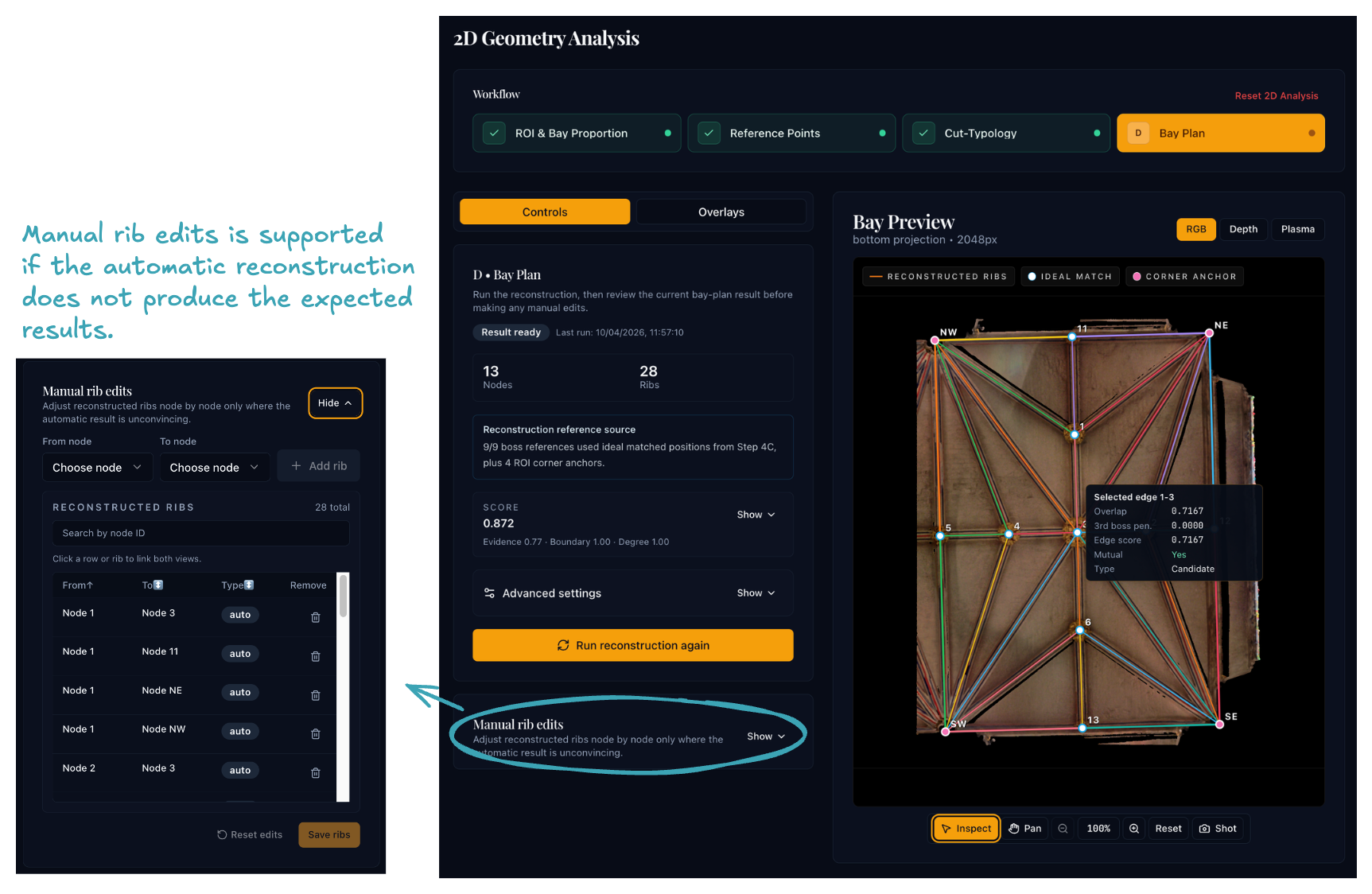
Step 4D: Bay-Plan Reconstruction¶

Purpose¶

This final Step 4 sub-stage reconstructs the bay plan from the ROI, reference points, matching results, and segmentation masks.

Workflow¶

1. Review the reconstruction settings¶

Start with the default settings. Tune the advanced parameters below only if the defaults do not produce satisfactory results.

Parameter	Description
Reconstruction mode	angular_nearest (default) or delaunay
Angle tolerance	Minimum angular separation between candidate directions per node
Candidate min score	Rib-mask overlap threshold for accepting a candidate edge
Candidate max distance	Maximum (u, v) distance between nodes for a candidate edge
Corridor width	Pixel width of the rib-mask overlap corridor
Min / max node degree	Degree bounds for the graph-selection and repair passes
Boundary tolerance	(u, v) margin for classifying a node as lying on the ROI boundary
Enforce planarity	Whether to reject edges that would cross existing selected edges

2. Run reconstruction¶

The backend loads the saved node points from sub-stage 4B (preferring ideal template positions from 4C where available) and the grouped rib-segmentation mask. It then:

1. Generates candidate edges — for each node, finds nearby neighbours in distinct directions and scores each edge by rib-mask overlap.¹ An alternative Delaunay mode is available when mask evidence is weak.²
2. Selects the final graph — adds boundary edges first, then greedily adds candidates in score order (subject to degree limits and optional planarity), and repairs any under-connected nodes.
3. Scores the result on four weighted components:

Component	Weight	Description
Edge evidence	55 %	Mean rib-mask overlap score of non-boundary edges
Boundary coverage	20 %	Proportion of mandatory boundary edges present
Degree satisfaction	15 %	Proportion of nodes within the degree bounds
Mutual support	10 %	Proportion of edges confirmed in both directions

3. Inspect and edit¶

• Compare the graph against the underlying projection and masks using the layer toggles.
• Add missing edges or remove wrong ones manually. Manual edits are saved alongside the computed graph.

If the graph has obvious errors, try the following before editing manually:

• Lower candidate min score to recover missing edges in areas with weak rib-mask evidence.
• Raise max node degree if key junctions are losing edges.
• Lower candidate max distance if the graph connects nodes across the bay that should not be linked.
• Switch reconstruction mode to delaunay for comparison — if it produces a cleaner graph, the rib-mask evidence may be too noisy for angular-nearest.

Why it matters¶

The bay plan is the main 2D output: Step 5 reprojects it into three-dimensional space. Errors here — missing ribs, false connections, misplaced nodes — propagate into all downstream 3D geometry.

Before moving on¶

Before leaving Step 4 you should have:

• a bay plan whose edges match the visible rib pattern
• any necessary manual corrections applied
• a saved result ready for Step 5